(U-Net) 모델 분석 및 Pytorch로 구현 - 1
오늘은 Biomedical 분야 Semantic Segmentation을 위한 Convolutional network 인 U-Net에 대해 포스팅 하려고 합니다.
https://link.springer.com/content/pdf/10.1007/978-3-319-24574-4_28.pdf
(U-Net: Convolutional Networks for Biomedical Image Segmentation
Olaf Ronneberger, Philipp Fischer, and Thomas Brox)
U-Net의 구조
- U-Net의 구조는 아래와 같습니다.
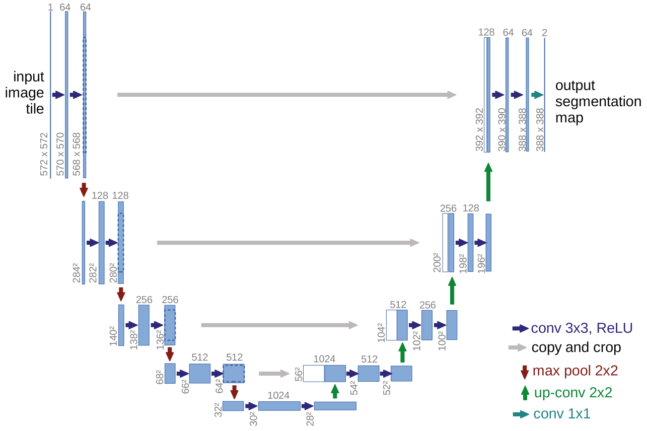
U-Net은 'Contracting path', 'Bottle Neck', 'Expanding path'로 구성되어있습니다.
'수축 단계(Contracting path)'
입력된 이미지에 아래 연산을 반복
1. Convolution( 3x3 kernel, stride : 1) X 2
2. Max Pooling( 2x2 kernel, stride : 2)
'전환 구간(Bottle neck)'
수축 단계를 거친 후 팽창 단계로 전환되는 구간
1. Convolution( 3x3 kernel, stride : 1) X 2
'팽창 단계(Expanding path)'
1. Up-Convolution( 2x2 kernel, stride : 2) 이후 같은 단계에 있는 Feature map을 합침
2. Convolution( 3x3 kernel, stride : 1) X 2
Feature map의 채널 수는 '이미지 입력', 'Max Pooling' , 'Up-Convolution' 이후 첫 'Convolution' 연산을 수행할 때
변화가 생깁니다.
각 연산을 수행 할 때 padding을 추가하지 않으므로 Feature map의 크기는 점점 작아지게 됩니다.
Pytorch로 구현한 U-Net 모델
class UNet(torch.nn.Module):
    def __init__(self):
        super().__init__()

		# Convolution, Batch Normalization, ReLU 연산을 합친 함수
        def CBR2d(input_channel, output_channel, kernel_size=3, stride=1):
            layer = nn.Sequential(
                nn.Conv2d(input_channel, output_channel, kernel_size=kernel_size, stride=stride),
                nn.BatchNorm2d(num_features=output_channel),
                nn.ReLU()
            )
            return layer

		# Contracting path
        # 572x572x1 => 568x568x64
        self.conv1 = nn.Sequential(
            CBR2d(1, 64, 3, 1),
            CBR2d(64, 64, 3, 1)
        )
		# 568x568x64 => 284x284x64
        self.pool1 = nn.MaxPool2d(kernel_size=2, stride=2)


		# 284x284x64 => 280x280x128
        self.conv2 = nn.Sequential(
            CBR2d(64, 128, 3, 1),
            CBR2d(128, 128, 3, 1)
        )
		# 280x280x128 => 140x140x128
        self.pool2 = nn.MaxPool2d(kernel_size=2, stride=2)


		# 140x140x128 => 136x136x256
        self.conv3 = nn.Sequential(
            CBR2d(128, 256, 3, 1),
            CBR2d(256, 256, 3, 1)
        )
		# 136x136x256 => 68x68x256
        self.pool3 = nn.MaxPool2d(kernel_size=2, stride=2)


		# 68x68x256 => 64x64x512
        # Contracting path 마지막에 Dropout 적용
        self.conv4 = nn.Sequential(
            CBR2d(256, 512, 3, 1),
            CBR2d(512, 512, 3, 1),
            nn.Dropout(p=0.5)
        )
		# 64x64x512 => 32x32x512
        self.pool4 = nn.MaxPool2d(kernel_size=2, stride=2)
		# Contracting path 끝


        # Bottlneck 구간
        # 32x32x512 => 28x28x1024
        self.bottleNeck = nn.Sequential(
            CBR2d(512, 1024, 3, 1),
            CBR2d(1024, 1024, 3, 1),
        )
		# Bottlneck 구간 끝


		# Expanding path
        # channel 수를 감소 시키며 Up-Convolution
		# 28x28x1024 => 56x56x512
        self.upconv1 = nn.ConvTranspose2d(in_channels=1024, out_channels=512, kernel_size=2, stride=2)


		# Up-Convolution 이후 channel = 512
        # Contracting path 중 같은 단계의 Feature map을 가져와 Up-Convolution 결과의 Feature map과 Concat 연산
        # => channel = 1024 가 됩니다.
        # forward 부분을 참고해주세요
        # 56x56x1024 => 52x52x512
        self.ex_conv1 = nn.Sequential(
            CBR2d(1024, 512, 3, 1),
            CBR2d(512, 512, 3, 1)
        )

		# 52x52x512 => 104x104x256
        self.upconv2 = nn.ConvTranspose2d(in_channels=512, out_channels=256, kernel_size=2, stride=2)

		# 104x104x512 => 100x100x256
        self.ex_conv2 = nn.Sequential(
            CBR2d(512, 256, 3, 1),
            CBR2d(256, 256, 3, 1)
        )

		# 100x100x256 => 200x200x128
        self.upconv3 = nn.ConvTranspose2d(in_channels=256, out_channels=128, kernel_size=2, stride=2)

		# 200x200x256 => 196x196x128
        self.ex_conv3 = nn.Sequential(
            CBR2d(256, 128, 3, 1),
            CBR2d(128, 128, 3, 1)
        )

		# 196x196x128 => 392x392x64
        self.upconv4 = nn.ConvTranspose2d(in_channels=128, out_channels=64, kernel_size=2, stride=2)

		# 392x392x128 => 388x388x64
        self.ex_conv4 = nn.Sequential(
            CBR2d(128, 64, 3, 1),
            CBR2d(64, 64, 3, 1),

        )

		# 논문 구조상 output = 2 channel
	    # train 데이터에서 세포 / 배경을 검출하는것이 목표여서 class_num = 1로 지정
		# 388x388x64 => 388x388x1
        self.fc = nn.Conv2d(64, 1, kernel_size=1, stride=1)


    def forward(self, x):
    	# Contracting path
        # 572x572x1 => 568x568x64
        layer1 = self.conv1(x)

        # Max Pooling
        # 568x568x64 => 284x284x64
        out = self.pool1(layer1)

		# 284x284x64 => 280x280x128
        layer2 = self.conv2(out)

        # Max Pooling
        # 280x280x128 => 140x140x128
        out = self.pool2(layer2)

		# 140x140x128 => 136x136x256
        layer3 = self.conv3(out)

        # Max Pooling
        # 136x136x256 => 68x68x256
        out = self.pool3(layer3)

		# 68x68x256 => 64x64x512
        layer4 = self.conv4(out)

        # Max Pooling
        # 64x64x512 => 32x32x512
        out = self.pool4(layer4)

		# bottleneck
        # 32x32x512 => 28x28x1024
        bottleNeck = self.bottleNeck(out)

		# Expanding path
        # 28x28x1024 => 56x56x512
        upconv1 = self.upconv1(bottleNeck)

        # Contracting path 중 같은 단계의 Feature map을 가져와 합침
        # Up-Convolution 결과의 Feature map size 만큼 CenterCrop 하여 Concat 연산
        # 56x56x512 => 56x56x1024
        cat1 = torch.cat((transforms.CenterCrop((upconv1.shape[2], upconv1.shape[3]))(layer4), upconv1), dim=1)

        # 56x56x1024 => 52x52x512
        ex_layer1 = self.ex_conv1(cat1)

		# 52x52x512 => 104x104x256
        upconv2 = self.upconv2(ex_layer1)

        # Contracting path 중 같은 단계의 Feature map을 가져와 합침
        # Up-Convolution 결과의 Feature map size 만큼 CenterCrop 하여 Concat 연산
        # 104x104x256 => 104x104x512
        cat2 = torch.cat((transforms.CenterCrop((upconv2.shape[2], upconv2.shape[3]))(layer3), upconv2), dim=1)

        # 104x104x512 => 100x100x256
        ex_layer2 = self.ex_conv2(cat2)

		# 100x100x256 => 200x200x128
        upconv3 = self.upconv3(ex_layer2)

        # Contracting path 중 같은 단계의 Feature map을 가져와 합침
        # Up-Convolution 결과의 Feature map size 만큼 CenterCrop 하여 Concat 연산
        # 200x200x128 => 200x200x256
        cat3 = torch.cat((transforms.CenterCrop((upconv3.shape[2], upconv3.shape[3]))(layer2), upconv3), dim=1)

        # 200x200x256 => 196x196x128
        ex_layer3 = self.ex_conv3(cat3)

		# 196x196x128=> 392x392x64
        upconv4 = self.upconv4(ex_layer3)

        # Contracting path 중 같은 단계의 Feature map을 가져와 합침
        # Up-Convolution 결과의 Feature map size 만큼 CenterCrop 하여 Concat 연산
        # 392x392x64 => 392x392x128
        cat4 = torch.cat((transforms.CenterCrop((upconv4.shape[2], upconv4.shape[3]))(layer1), upconv4), dim=1)

        # 392x392x128 => 388x388x64
        out = self.ex_conv4(cat4)

		# 388x388x64 => 388x388x1
        out = self.fc(out)
        return out
해당 모델을 학습하는 Pytorch 코드는 다음 포스팅에 올리도록 하겠습니다.
모델 학습시 입력 이미지(512x512)가 모델을 거친 후 (324x324) size의 이미지가 출력됩니다.
- label 데이터의 324x324를 Center Crop 하여 학습을 진행하였습니다.
그리고 모델을 거친 후에 입력 이미지와 같은 크기의 결과를 얻기 위해
논문에 나와있는 'Mirroring Extrapolation'을 적용하고 'Overlap-tile strategy' 기법을 이용하여 코드 구현중입니다.
이 부분도 구현을 마치게 되면 포스팅 하도록 하겠습니다.
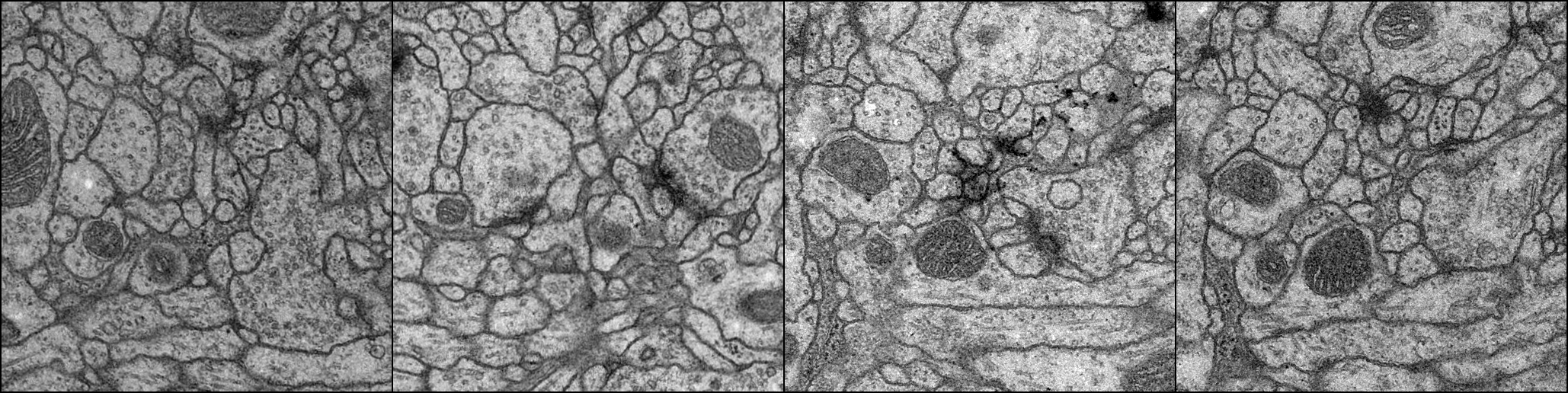
Training dataset은 ISBI 2012 em image segmentation 대회에서 사용한 이미지 데이터 셋 (30장)을 사용하였습니다.
training data = 24장
validation data = 6장
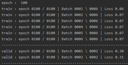
Epoch : 100회
Batch size = 4
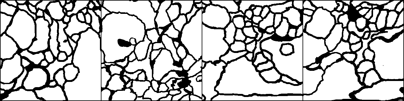
학습 결과는 아래와 같습니다.
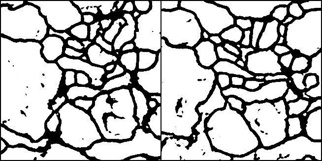
Training set 결과
Input(512 x 512)
Label(324 x 324 CenterCrop)
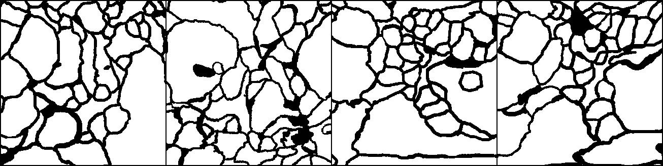
Output(324 x 324)
Validation set 결과
Input(512 x 512)
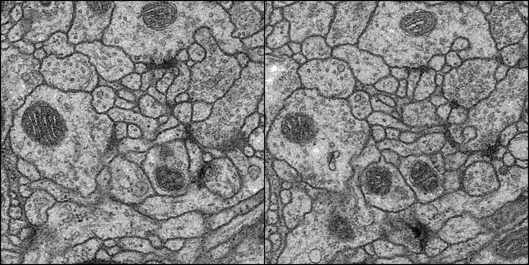
Label(324 x 324 CenterCrop)
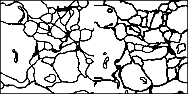
Output(324 x 324)